Create a fit vs exposure(s)plot — ggresponseexpdist • ggquickeda

Produces a fit as per model_type plot with a facettable exposures/quantiles/distributions in ggplot2

Usage

ggresponseexpdist(
  data = dplyr::filter(logistic_data, !is.na(ICGI)),
  response = "response",
  endpoint = "Endpoint",
  model_type = c("loess", "linear", "logistic", "none"),
  DOSE = "DOSE",
  color_fill = "DOSE",
  fit_by_color_fill = FALSE,
  exposure_metrics = c("AUC", "CMAX"),
  exposure_metric_split = c("median", "tertile", "quartile", "none"),
  exposure_metric_soc_value = -99,
  exposure_metric_plac_value = 0,
  exposure_metric_soc_name = "SOC",
  exposure_metric_plac_name = "Placebo",
  exposure_distribution = c("distributions", "lineranges", "boxplots", "none"),
  exposure_distribution_percent = c("none", "%", "N (%)", "N"),
  exposure_distribution_Ntotal = c("none", "left", "right"),
  exposure_distribution_percent_text_size = 5,
  dose_plac_value = "Placebo",
  xlab = "Exposure Values",
  ylab = "Response",
  points_alpha = 0.2,
  points_show = TRUE,
  mean_obs_byexptile = TRUE,
  mean_obs_byexptile_plac = TRUE,
  mean_obs_byexptile_text_size = 5,
  mean_obs_byexptile_group = "none",
  mean_obs_bydose = FALSE,
  mean_obs_bydose_plac = FALSE,
  mean_obs_bydose_text_size = 5,
  N_byexptile_ypos = c("with means", "top", "bottom", "none"),
  N_bydose_ypos = c("with means", "top", "bottom", "none"),
  N_text_size = 5,
  N_text_sep = NULL,
  binlimits_show = TRUE,
  binlimits_text_size = 5,
  binlimits_ypos = 0,
  binlimits_color = "#B3B3B380",
  dist_position_scaler = 0.2,
  dist_offset = 0,
  dist_scale = 0.9,
  lineranges_ypos = NULL,
  lineranges_dodge = NULL,
  lineranges_doselabel = FALSE,
  lineranges_Ntotal = c("none", "left", "right"),
  proj_bydose = FALSE,
  yproj = FALSE,
  yproj_xpos = 0,
  yproj_dodge = 0.2,
  yaxis_position = c("left", "right"),
  facet_formula = NULL,
  theme_certara = TRUE,
  color_legend_title = "",
  fill_legend_title = "",
  linetype_legend_title = "",
  shape_legend_title = "",
  combine_fill_linetype_legend = TRUE,
  legend_order = c("model", "color", "linetype", "shape"),
  return_list = FALSE
)

Arguments

data: Data to use with multiple endpoints stacked into response (values), Endpoint(endpoint name)
response: name of the column holding the response values
endpoint: name of the column holding the name/key of the endpoint default to Endpoint
model_type: type of the trend fit one of "loess", "linear", "logistic", "none"
DOSE: name of the column holding the DOSE/regimen values default to DOSE should be a factor
color_fill: name of the column to be used for color/fill default to DOSE column should be a factor
fit_by_color_fill: split fit by color/fill? default FALSE
exposure_metrics: name(s) of the column(s) to be stacked into expname exptile and split into exposure_metric_split
exposure_metric_split: one of "median", "tertile", "quartile", "none"
exposure_metric_soc_value: special exposure code for standard of care default -99
exposure_metric_plac_value: special exposure code for placebo default 0
exposure_metric_soc_name: soc name default to "soc"
exposure_metric_plac_name: placebo name default to "placebo"
exposure_distribution: one of distributions, lineranges, boxplots or none
exposure_distribution_percent: show N/percent of distribution between binlimits one of "%", "N (%)","N","none"
exposure_distribution_Ntotal: show Ntotal by dose level next to the distribution one of "left","right","none"
exposure_distribution_percent_text_size: distribution percentages text size default to 5
dose_plac_value: string identifying placebo in DOSE column
xlab: text to be used as x axis label
ylab: text to be used as y axis label
points_alpha: alpha transparency for points
points_show: show the observations TRUE/FALSE
mean_obs_byexptile: observed mean by exptile TRUE/FALSE
mean_obs_byexptile_plac: observed mean by exptile placebo TRUE/FALSE
mean_obs_byexptile_text_size: by exptile mean text size default to 5
mean_obs_byexptile_group: additional grouping for exptile means default none
mean_obs_bydose: observed mean by dose TRUE/FALSE
mean_obs_bydose_plac: observed mean by placebo dose TRUE/FALSE
mean_obs_bydose_text_size: by dose mean text size default to 5
N_byexptile_ypos: N responders/Ntotal y position by exptile one of with means top bottom none
N_bydose_ypos: N responders/Ntotal y position by dose/color one of with means top bottom none
N_text_size: N responders/Ntotal text size default to 5
N_text_sep: character string to separate N responders/Ntotal or N/mean defaults to / otherwise \n
binlimits_show: show the binlimits vertical lines TRUE/FALSE
binlimits_text_size: binlimits text size default to 5
binlimits_ypos: binlimits y position default to -Inf
binlimits_color: binlimits text color default to alpha("gray70",0.5)
dist_position_scaler: space occupied by the distribution default to 0.2
dist_offset: offset where the distribution position starts default to 0
dist_scale: scaling parameter for ggridges default to 0.9
lineranges_ypos: where to put the lineranges -1
lineranges_dodge: lineranges vertical dodge value 1
lineranges_doselabel: TRUE/FALSE
lineranges_Ntotal: show Ntotal by dose level next to the lineranges one of "left","right","none"
proj_bydose: project the predictions on the fit curve TRUE/FALSE
yproj: project the predictions on y axis TRUE/FALSE
yproj_xpos: y projection x position 0
yproj_dodge: y projection dodge value 0.2
yaxis_position: where to put y axis "left" or "right"
facet_formula: facet formula to be use otherwise endpoint ~ expname
theme_certara: apply certara colors and format for strips and default colour/fill
color_legend_title: text for colour legend title
fill_legend_title: text for fill legend title
linetype_legend_title: text for linetype legend title
shape_legend_title: text for shape legend title
combine_fill_linetype_legend: defaults to true
legend_order: Legend order. A four-element vector with the following items ordered in your desired order: "model", "color", "linetype", "shape". if an item is absent the legend will be omitted.
return_list: What to return if True a list of the datasets and plot is returned instead of only the plot

Examples

# Example 1
library(ggplot2)
effICGI <- logistic_data |>
dplyr::filter(!is.na(ICGI))|>
dplyr::filter(!is.na(AUC))
effICGI$DOSE <- factor(effICGI$DOSE,
                      levels=c("0", "600", "1200","1800","2400"),
                      labels=c("Placebo", "600 mg", "1200 mg","1800 mg","2400 mg"))
effICGI$STUDY <- factor(effICGI$STUDY)    
effICGI$ICGI2 <- effICGI$ICGI
effICGI <- tidyr::gather(effICGI,Endpoint,response,ICGI,ICGI2)

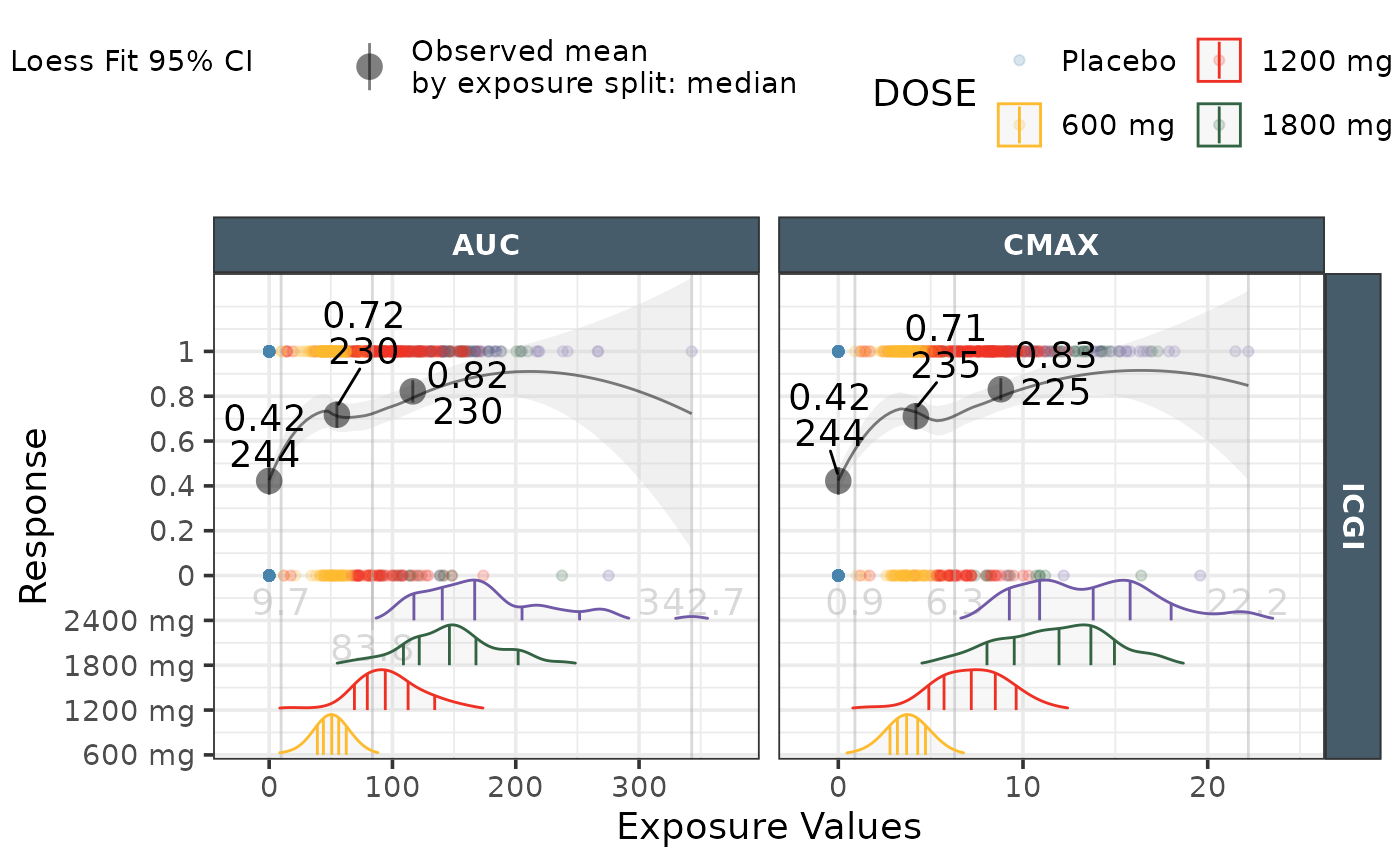
ggresponseexpdist(data = effICGI |>
dplyr::filter(Endpoint=="ICGI"),
model_type = "loess",
exposure_metrics = c("AUC","CMAX"),
legend_order = c("color","shape","model"),
color_legend_title ="Dose\nLevels")
#> Joining with `by = join_by(loopvariable, DOSE, quant_10)`
#> Joining with `by = join_by(loopvariable, DOSE, quant_90)`
#> Joining with `by = join_by(loopvariable, DOSE, quant_25)`
#> Joining with `by = join_by(loopvariable, DOSE, quant_75)`
#> Joining with `by = join_by(loopvariable, DOSE, medexp)`
#> Joining with `by = join_by(loopvariable, DOSE, quant_10)`
#> Joining with `by = join_by(loopvariable, DOSE, quant_90)`
#> Joining with `by = join_by(loopvariable, DOSE, quant_25)`
#> Joining with `by = join_by(loopvariable, DOSE, quant_75)`
#> Joining with `by = join_by(loopvariable, DOSE, medexp)`
#> `geom_smooth()` using formula = 'y ~ x'
#> `geom_smooth()` using formula = 'y ~ x'
#> Picking joint bandwidth of 11.7
#> Picking joint bandwidth of 0.934
#> Warning: Removed 488 rows containing non-finite outside the scale range
#> (`stat_density_ridges()`).


# Example 2
ggresponseexpdist(data = effICGI |>
dplyr::filter(Endpoint=="ICGI"),
model_type = "logistic",
exposure_metrics = c("AUC","CMAX"),
exposure_distribution ="boxplots")
#> Joining with `by = join_by(loopvariable, DOSE, quant_10)`
#> Joining with `by = join_by(loopvariable, DOSE, quant_90)`
#> Joining with `by = join_by(loopvariable, DOSE, quant_25)`
#> Joining with `by = join_by(loopvariable, DOSE, quant_75)`
#> Joining with `by = join_by(loopvariable, DOSE, medexp)`
#> Joining with `by = join_by(loopvariable, DOSE, quant_10)`
#> Joining with `by = join_by(loopvariable, DOSE, quant_90)`
#> Joining with `by = join_by(loopvariable, DOSE, quant_25)`
#> Joining with `by = join_by(loopvariable, DOSE, quant_75)`
#> Joining with `by = join_by(loopvariable, DOSE, medexp)`
#> `geom_smooth()` using formula = 'y ~ x'
#> `geom_smooth()` using formula = 'y ~ x'
#> Warning: Removed 488 rows containing non-finite outside the scale range
#> (`stat_boxplot()`).


# Example 3
ggresponseexpdist(data = effICGI|>
dplyr::filter(Endpoint=="ICGI"),
model_type = "linear",
exposure_metrics = c("AUC","WT"),
exposure_distribution ="lineranges")
#> Joining with `by = join_by(loopvariable, DOSE, quant_10)`
#> Joining with `by = join_by(loopvariable, DOSE, quant_90)`
#> Joining with `by = join_by(loopvariable, DOSE, quant_25)`
#> Joining with `by = join_by(loopvariable, DOSE, quant_75)`
#> Joining with `by = join_by(loopvariable, DOSE, medexp)`
#> Joining with `by = join_by(loopvariable, DOSE, quant_10)`
#> Joining with `by = join_by(loopvariable, DOSE, quant_90)`
#> Joining with `by = join_by(loopvariable, DOSE, quant_25)`
#> Joining with `by = join_by(loopvariable, DOSE, quant_75)`
#> Joining with `by = join_by(loopvariable, DOSE, medexp)`
#> `geom_smooth()` using formula = 'y ~ x'
#> Warning: In lm.wfit(x, y, w, offset = offset, singular.ok = singular.ok, 
#>     ...) :
#>  extra argument ‘family’ will be disregarded
#> Warning: In lm.wfit(x, y, w, offset = offset, singular.ok = singular.ok, 
#>     ...) :
#>  extra argument ‘family’ will be disregarded
#> `geom_smooth()` using formula = 'y ~ x'
#> Warning: In lm.wfit(x, y, w, offset = offset, singular.ok = singular.ok, 
#>     ...) :
#>  extra argument ‘family’ will be disregarded
#> Warning: In lm.wfit(x, y, w, offset = offset, singular.ok = singular.ok, 
#>     ...) :
#>  extra argument ‘family’ will be disregarded


# Example 4
ggresponseexpdist(data = effICGI |>
                 dplyr::filter(Endpoint=="ICGI"),
                 response = "response",
                 endpoint = "Endpoint",
                 model_type = "loess",
                 DOSE = "DOSE",
                 color_fill = "DOSE",
                 exposure_metrics = c("AUC","CMAX"),
                 exposure_metric_split = c("tertile"),
                 exposure_metric_soc_value = -99,
                 exposure_metric_plac_value = 0,
                 exposure_distribution ="distributions",
                 exposure_distribution_Ntotal="right",
                 N_byexptile_ypos = "top",
                 mean_obs_bydose = TRUE,
                 mean_obs_bydose_text_size = 0,
                 mean_obs_byexptile_text_size = 5,
                 N_bydose_ypos = "none",
                 N_text_sep = "/",
                 binlimits_color = "#475c6b",
                 binlimits_ypos = 0.2,
                 points_alpha= 0.1)
#> Joining with `by = join_by(loopvariable, DOSE, quant_10)`
#> Joining with `by = join_by(loopvariable, DOSE, quant_90)`
#> Joining with `by = join_by(loopvariable, DOSE, quant_25)`
#> Joining with `by = join_by(loopvariable, DOSE, quant_75)`
#> Joining with `by = join_by(loopvariable, DOSE, medexp)`
#> Joining with `by = join_by(loopvariable, DOSE, quant_10)`
#> Joining with `by = join_by(loopvariable, DOSE, quant_90)`
#> Joining with `by = join_by(loopvariable, DOSE, quant_25)`
#> Joining with `by = join_by(loopvariable, DOSE, quant_75)`
#> Joining with `by = join_by(loopvariable, DOSE, medexp)`
#> `geom_smooth()` using formula = 'y ~ x'
#> `geom_smooth()` using formula = 'y ~ x'
#> Picking joint bandwidth of 11.7
#> Picking joint bandwidth of 0.934
#> Warning: Removed 488 rows containing non-finite outside the scale range
#> (`stat_density_ridges()`).

                 
if (FALSE) { # \dontrun{
# Example 5 
effICGI <- logistic_data |>
dplyr::filter(!is.na(ICGI))|>
dplyr::filter(!is.na(AUC))
effICGI$DOSE <- factor(effICGI$DOSE,
                      levels=c("0", "600", "1200","1800","2400"),
                      labels=c("Placebo", "600 mg", "1200 mg","1800 mg","2400 mg"))
effICGI$STUDY <- factor(effICGI$STUDY)
effICGI$ICGI2 <- ifelse(effICGI$ICGI7 < 4,1,0)
effICGI$ICGI3 <- ifelse(effICGI$ICGI7 < 5,1,0)

effICGI <- tidyr::gather(effICGI,Endpoint,response,ICGI,ICGI2,ICGI3)
effICGI$endpointcol2 <- effICGI$Endpoint
effICGI$endpointcol3 <- effICGI$Endpoint

ggresponseexpdist(data = effICGI,
                  points_show = FALSE,
                  exposure_metrics = c("AUC"),
                  exposure_distribution ="lineranges",
                  color_fill = "endpointcol2",
                  model_type = "logistic",                   
                  fit_by_color_fill = TRUE,
                  mean_obs_byexptile_text_size = 0,
                  mean_obs_byexptile_group="endpointcol3",
                  facet_formula = Endpoint~expname,
                  N_byexptile_ypos = "none",
                  binlimits_text_size = 0
                 )+
                  ggplot2::facet_grid(expname~Endpoint,margin="Endpoint")

# Example 6 retrun a list and customize
plist <- ggresponseexpdist(data = effICGI |>
dplyr::filter(Endpoint=="ICGI"),
model_type = "logistic",
mean_obs_byexptile = TRUE,
N_byexptile_ypos = "none",
mean_obs_byexptile_text_size = 4,
binlimits_ypos = -Inf,
exposure_metric_split = "tertile",
exposure_metrics = c("AUC"),
return_list = TRUE)
byexptileinformation <- plist[[7]]
plotwihoutlabels <- plist[[9]]

#construct text label
byexptileinformation <- byexptileinformation %>%
 dplyr::group_by(exptile,expname)%>%
 dplyr::mutate(meanbin = mean(c(minexp,maxexp))) %>%
 dplyr::mutate(label = ifelse(exptile!="Placebo",
                       paste0(exptile,"\n","[",round(minexp,0),"-",round(maxexp,0),"]",
                              "\n",N,"\n",Ntot),
                       paste0(exptile,"\n","",
                              "\n",N,"\n",Ntot)),
        x_pos = ifelse(exptile=="Placebo",-25,meanbin )
 )

plotwihoutlabels +
 geom_text(data=byexptileinformation,size = 3,
           aes(x=x_pos ,label=label,y = 0.5),
           inherit.aes = FALSE,
           vjust= 1, hjust = 0.5)+
 geom_text(data=data.frame(
   label="exposure ntile\n[min-max]\nN responders\nN Total"),size = 3,
   x=Inf,y = 0.5,
   aes(label=label),inherit.aes = FALSE,
   vjust= 1, hjust = 1)+
 facet_wrap(~expname,ncol=2,scales = "free_x")
} # }