Applications of the Delta Method in Pharmacometrics

Methods
visualization
uncertainty
Author

Samer Mouksassi

Published

December 1, 2025

In pharmacometrics models we often have model parameters modeled as a function of one or multiple covariates:

\[CL = \color{blue}{POPCL}\times\left(\frac{\color{green}{Weight}}{70}\right)^{\color{blue}{dWTdCL}}\times\left(\frac{\color{green}{Age}}{\color{green}{Age}+\color{blue}{Age50}}\right)\times e^{\eta CL}\]

In this example the parameter clearance (CL) has two covariates effects:

The ηCL denotes the individual deviations from the population (random effects) which assumes that the population CL is log normally distributed.

Common software will estimate the fixed effects, random effects variances and provide the associated standard errors. For example we would get POPCL = 42 ± 1.73 L/h, the weight power effect = 1.0078 ± 0.17 and age maturation Age50 = 4.84 ± 2.90 years. What would be the Cl for a 3 years old 14 kg kid? 42(14/70)^1.0078(3/(3+4.84)) = 3.17 L/h. What would be its standard error?

Also, we often want to report the CV% of the log normal distribution expressed as:

\[CV(\%)=\sqrt{\left(e^{\omega^2}-1\right)}\] Again, what would be the standard error of the CV%?

The delta method is a statistical technique to approximate the standard error of a function of an estimator, such as a ratio or the log odds ratio or the inverse logit of a constrained parameter, using a first-order Taylor series expansion. It’s especially useful when the function involves more than one parameter and/or the equation is complex such as there is no straightforward analytically computed solution. It relies on the original variable(s), the function form and the partial derivative of the function with respect to the parameters and the variance covariance matrix of the involved parameters. It has been used in multiple fields, including pharmacometrics, that the delta method matches the gold standard (simulation with uncertainty) even with longitudinal model based meta-analysis (MBMA) nonlinear models. Also, in this important paper from the FDA entitled Clarification on Precision Criteria to Derive Sample Size When Designing Pediatric Pharmacokinetic Studies R code to compute the delta method for derived variables was provided in APPENDIX 3. R code for delta method to estimate standard error for a derived variable

\[log(CL) = \color{blue}{3.7421} + \color{blue}{1.0078}\times log\left( \frac { \color{green}{Weight}} {70}\right)+log\left(\color{green}{Age}/(\color{green}{Age}+4.8422)\right)\] Note that the log of the equation above was estimated and used:

# Assume covariate model CL=theta1*(wt/70)** theta2*age/(age+theta3) and
# Log of CL was modeled as LCL=thetap1+theta2*log(wt/70)+log(age/(age+theta3))
#input parameter estimates
 thetap1=3.7421
 theta2=1.0078
 theta3=4.8422
#input variance-covariance matrix for the 3 parametersabove
 covp3=matrix(
   c(0.29810, 0.05782, 1.27120,
     0.05782, 0.02921, 0.02073,
     1.27120, 0.02073, 8.42210),
   nrow=3, byrow=T)
  #define the weight and age combination for SE estima-tion
 wt=14
 age=3
 #define covariate model in R
 f <- function(x,y,z) x + y*log(wt/70) + log(age/(age+z))
 df<- deriv(body(f), c("x","y","z"))
 x=thetap1
 y=theta2
 z=theta3
 out=eval(df)
 dfout=attr(out,"gradient")
 varlcl=dfout%*%covp3%*%t(dfout)
SElcl=sqrt(varlcl)
SElcl
           [,1]
[1,] 0.09436884

The code above works, but it is easier to use the R package msm which has a streamlined general deltamethod function of which I have a copy in my own package coveffectsplot. The only difference in mine is explicitly adding the evaluation environment which was necessary for the function to properly work in an R Shiny App. The deltamethod function source code:

deltamethod <-  function (g, mean, cov, ses = TRUE, envir = parent.frame()) 
{
    cov <- as.matrix(cov)
    n <- length(mean)
    if (!is.list(g)) 
        g <- list(g)
    if ((dim(cov)[1] != n) || (dim(cov)[2] != n)) 
        stop(paste("Covariances should be a ", n, " by ", n, 
            " matrix"))
    syms <- paste("x", 1:n, sep = "")
    for (i in 1:n) assign(syms[i], mean[i])
    gdashmu <- t(sapply(g, function(form) {
        as.numeric(attr(eval(deriv(form, syms)), "gradient"))
    }))
    new.covar <- gdashmu %*% cov %*% t(gdashmu)
    if (ses) {
        new.se <- sqrt(diag(new.covar))
        new.se
    }
    else new.covar
}

I load coveffectsplot and use the deltamethod function to recompute SElcl exactly matching the result above note how the function should refer to the parameters as x1, x2, …, etc.

library(coveffectsplot)
 deltamethod (~ x1 + x2*log(wt/70) + log(age/(age+x3)),
              c(thetap1,theta2,theta3), covp3) 
[1] 0.09436884

As expected, I get the same answer = 0.09436884.

I have used this function in several pediatric filings/approvals. One advantage of the deltamethod is that it can be very fast and suitable for interactive Shiny Application to compute confidence intervals around effects or hazard ratios for an example refer to this paper Total Kidney Volume Is a Prognostic Biomarker of Renal Function Decline and Progression to End-Stage Renal Disease in Patients With Autosomal Dominant Polycystic Kidney Disease that had a Shiny App deployed here. This was part of the qualification of kidney volume as a Drug Development Tool for which I will write a separate post in the future. The FDA review can be consulted at this link.

Back to the random effect variance expressed as CV% standard error we can use the same code and function to compute a standard error for a transformation of the original estimated variance:

 omegaCL<-  0.42
 covOMEGA=matrix( c(0.2),nrow=1, byrow=T)
 sqrt(exp(omegaCL)-1) # formula for CV of a log normal
[1] 0.7224691

The CV% is computed to be ~72.2 % with a standard error of: 0.4710526

 deltamethod (~  sqrt(exp(x1)-1), c(omegaCL), covOMEGA)
[1] 0.4710526

Another approach, albeit more time consuming, is to simulate the distribution using enough n samples and then compute the CV% using its formula: sd(x)/mean(x) which will exactly match the analytical formula for this relatively simple case:

set.seed(165413)
omegaCL<-  0.42
etaCL<- exp(rnorm(10000000,mean=0,sd=0.42^0.5))
sd(etaCL)/mean(etaCL)
[1] 0.7222556
sqrt(exp(omegaCL)-1)
[1] 0.7224691

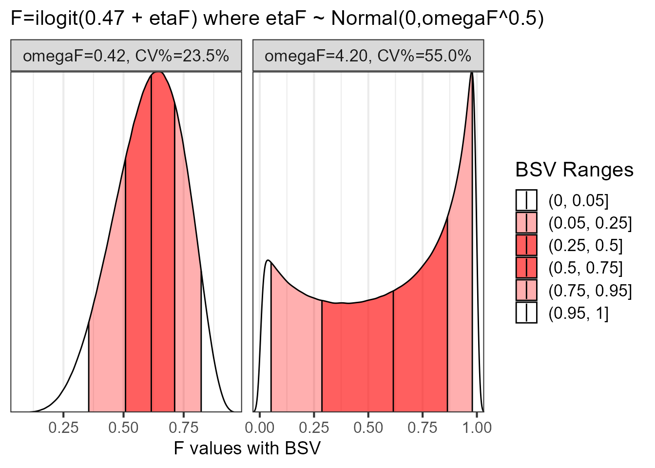
What if we have a more complex random effect model? Say an inverse logit transformation to constrain a parameter like bioavailbility between 0 and 1? Let us explore it with simulation !

library(ggridges)
library(ggplot2)
set.seed(165413)
Flogit <- 0.47
Fvalue<- exp(Flogit)/(1+exp(Flogit))
omegaF <-  0.42
etaF <- rnorm(10000000,mean=0,sd=omegaF^0.5)
set.seed(165413)
etaF2 <- rnorm(10000000,mean=0,sd=(10*omegaF)^0.5)
Feta <- exp(Flogit+etaF)/(1+exp(Flogit+etaF))
Feta2 <- exp(Flogit+etaF2)/(1+exp(Flogit+etaF2))

The omegaF = 0.42 translates to a %CV of ~23.5%

100*sd(Feta)/mean(Feta)
[1] 23.51329

When we multiply the omegaF by 10 = 4.2 the %CV becomes ~55.0%

100*sd(Feta2)/mean(Feta2)
[1] 55.04038

How appropriate is this summary? let us look at the distribution:

Fdataframe <- rbind(
  data.frame(Feta=Feta ,paramname="omegaF=0.42, CV%=23.5%"),
  data.frame(Feta=Feta2,paramname="omegaF=4.20, CV%=55.0%"))

  ggplot(data=Fdataframe, aes(
  x      = Feta,
  y      = paramname,
  fill   = factor(..quantile..),
  height = ..ndensity..)) +
  stat_density_ridges(
    geom="density_ridges_gradient", calc_ecdf=TRUE,
    quantile_lines=TRUE, rel_min_height=0.001, scale=0.9,
    quantiles=c(0.05, 0.25, 0.5, 0.75, 0.95)) +
  facet_wrap(~paramname,scales="free")+
  scale_fill_manual(
    name="BSV Ranges",
    values=c("white", "#FF000050", "#FF0000A0", "#FF0000A0", "#FF000050", "white"),
    labels = c("(0, 0.05]", "(0.05, 0.25]",
               "(0.25, 0.5]", "(0.5, 0.75]",
               "(0.75, 0.95]", "(0.95, 1]")) +
  theme_bw(base_size = 16) +
  theme(
    legend.position = "right",
    axis.text.y     = element_blank(),
    axis.ticks.y    = element_blank(),
    axis.title.y    = element_blank(),
    axis.text.x=element_text(size=12),
    axis.title.x=element_text(size=14)) +
  scale_x_continuous(breaks=c(0,0.25,0.5,0.75,1))+
  coord_cartesian(expand=FALSE)+
  labs(x="F values with BSV",
       subtitle="F=ilogit(0.47 + etaF) where etaF ~ Normal(0,omegaF^0.5)")

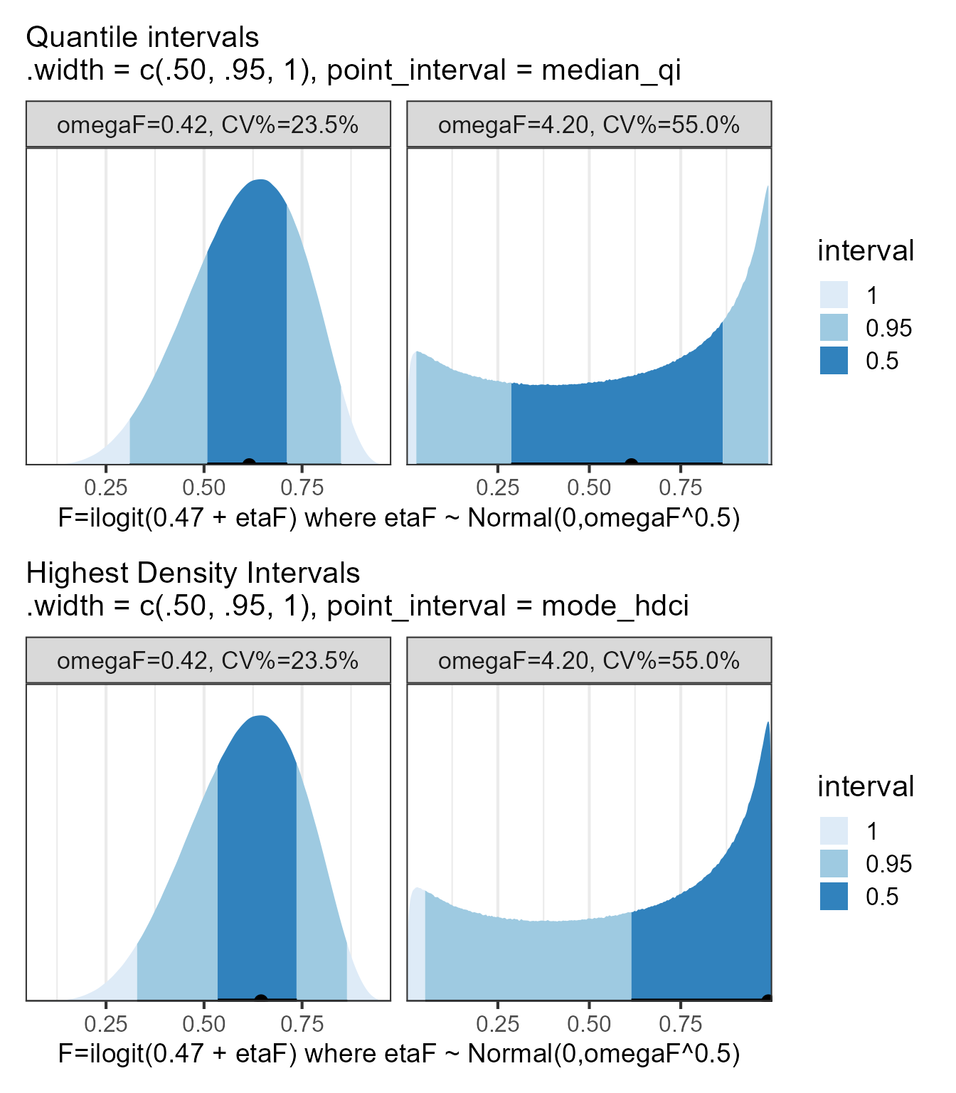
We can now see that when omegaF is 0.42 the distribution is a bit skewed with one mode while when the omegaF is 4.2 the distribution becomes multi-modal with a “weird” concentration of mass at 0 and 1. How representative is to “summarize” such a distribution with a CV%? isn’t it more useful to show the full distribution? This would help us in understanding the distribution shape and where will 50 or 90% of my patients be on the F scale. Another possible interval for highly skewed distribution are the highest density intervals which I will illustrate next using ggdist:

Code
library(ggdist)
library(patchwork)

 qi_plot <-  ggplot(Fdataframe,
         aes(y = paramname, x = Feta)) +
  stat_halfeye(aes(fill = after_stat(level)),
               point_interval = median_qi,
               .width = c(.50, .95, 1)) +
  scale_fill_brewer(na.translate = FALSE) +
  labs(x="F=ilogit(0.47 + etaF) where etaF ~ Normal(0,omegaF^0.5)",
    subtitle = "Quantile intervals\n.width = c(.50, .95, 1), point_interval = median_qi",
    fill = "interval"
  )+
facet_wrap(~paramname,scales="free")+
  theme_bw(base_size = 16) +
  theme(
    legend.position = "right",
    axis.text.y     = element_blank(),
    axis.ticks.y    = element_blank(),
    axis.title.y    = element_blank(),
    axis.text.x=element_text(size=12),
    axis.title.x=element_text(size=14)) +
  scale_x_continuous(breaks=c(0,0.25,0.5,0.75,1))+
  coord_cartesian(expand=FALSE)

hdi_plot  <-  ggplot(Fdataframe,
         aes(y = paramname, x = Feta)) +
  stat_halfeye(aes(fill = after_stat(level)),
               point_interval = mode_hdci,
               .width = c(.50, .95, 1)) +
  scale_fill_brewer(na.translate = FALSE) +
  labs(x="F=ilogit(0.47 + etaF) where etaF ~ Normal(0,omegaF^0.5)",
    subtitle = "Highest Density Intervals\n.width = c(.50, .95, 1), point_interval = mode_hdci",
    fill = "interval"
  )+
facet_wrap(~paramname,scales="free")+
  theme_bw(base_size = 16) +
  theme(
    legend.position = "right",
    axis.text.y     = element_blank(),
    axis.ticks.y    = element_blank(),
    axis.title.y    = element_blank(),
    axis.text.x=element_text(size=12),
    axis.title.x=element_text(size=14)) +
  scale_x_continuous(breaks=c(0,0.25,0.5,0.75,1))+
  coord_cartesian(expand=FALSE)  

qi_plot/hdi_plot

Next I compute the 50% intervals separately: Quantile Intervals median_qi

Code
library(dplyr)
Fdataframe %>%
  group_by(paramname)%>%
  median_qi(Feta, .width = c(0.5))
# A tibble: 2 × 7
  paramname               Feta .lower .upper .width .point .interval
  <chr>                  <dbl>  <dbl>  <dbl>  <dbl> <chr>  <chr>    
1 omegaF=0.42, CV%=23.5% 0.615  0.508  0.712    0.5 median qi       
2 omegaF=4.20, CV%=55.0% 0.615  0.286  0.864    0.5 median qi       

Highest Density Intervals: mode_hdi notice how we get multiple intervals one per mode for omegaF=4.20

Code
Fdataframe %>%
  group_by(paramname)%>%
  mode_hdi(Feta, .width = c(0.5))
# A tibble: 4 × 7
  paramname               Feta .lower .upper .width .point .interval
  <chr>                  <dbl>  <dbl>  <dbl>  <dbl> <chr>  <chr>    
1 omegaF=0.42, CV%=23.5% 0.645 0.535  0.737     0.5 mode   hdi      
2 omegaF=4.20, CV%=55.0% 0.989 0.0104 0.0982    0.5 mode   hdi      
3 omegaF=4.20, CV%=55.0% 0.989 0.712  0.714     0.5 mode   hdi      
4 omegaF=4.20, CV%=55.0% 0.989 0.717  1.000     0.5 mode   hdi      

Highest Density Intervals continuous: mode_hdci

Code
Fdataframe %>%
  group_by(paramname)%>%
  mode_hdci(Feta, .width = c(0.5))
# A tibble: 2 × 7
  paramname               Feta .lower .upper .width .point .interval
  <chr>                  <dbl>  <dbl>  <dbl>  <dbl> <chr>  <chr>    
1 omegaF=0.42, CV%=23.5% 0.645  0.535  0.737    0.5 mode   hdci     
2 omegaF=4.20, CV%=55.0% 0.989  0.615  1.000    0.5 mode   hdci     

When a distribution is asymmetrical, multimodal and/or with an important mass at the boundaries the quantile, the highest density and the highest density continuous intervals will significantly differ. I highly recommend to plot the data and to provide multiple interval types for such distributions.

In this post I have shown several examples/applications of the delta method to compute confidence intervals for a model statistic of interest that can be a function of one or multiple model parameters. I have also covered how to compute intervals around random effects distributions via simulations arguing that a single stat, such as CV%, can be misleading for non-symmetrical and/or multi-modal distributions using an inverse logit transformation of bioavailibility (F) as an example.