tkvt <- 1000* c(0.25,0.50, 0.75, 1.00, 1.25, 1.50, 1.75 ,2.00,3,4,5)
egfrt <- seq(50, 100,10)
aget <- 40* c(0.50, 0.75, 1.00, 1.25, 1.50)
matrixhr<- data.frame(
matrix(rep(NA,length(tkvt)+length(egfrt)+length(aget))*5,ncol=5,
nrow=length(tkvt)+length(egfrt)+length(aget)))
for (i in 1:length(egfrt) ){
matrixhr[i,1] <- "egft"
matrixhr[i,2] <- egfrt[i]
matrixhr[i,3:5] <- computerelativeHR(egfrt=egfrt[i],tkvt=1000,aget=40)
}
for (i in 1:length(tkvt) ){
matrixhr[i+length(egfrt),1] <- "tkvt"
matrixhr[i+length(egfrt),2] <- tkvt[i]
matrixhr[i+length(egfrt),3:5] <- computerelativeHR(egfrt=70,tkvt=tkvt[i],aget=40)
}
for (i in 1:length(aget) ){
matrixhr[i+length(egfrt)+length(tkvt),1] <- "aget"
matrixhr[i+length(egfrt)+length(tkvt),2] <- aget[i]
matrixhr[i+length(egfrt)+length(tkvt),3:5] <- computerelativeHR(egfrt=70,tkvt=1000,aget=aget[i])
}
names(matrixhr) <- c("cov","value","HR","LOW","HIGH")
refvalues <- data.frame(cov=c("egft","tkvt","aget"),ref=c(70,1000,40))
matrixhr<- left_join( matrixhr ,refvalues)
matrixhr<- matrixhr%>%
group_by(cov)%>%
mutate(valuecov= value/ref)
matrixhr$cov <- factor(matrixhr$cov)
levels( matrixhr$cov ) <- c("Age, ref=40 years",
"eGFR ref=70 mL/min/1.73m2",
"TKV ref=1000 mL")
covdistribution <- esrd[esrd$tkv_bsl<5100,c("tkv_bsl","age_bsl","egfr_bsl","status")]
covdistribution <- covdistribution[covdistribution$age_bsl>=20,c("tkv_bsl","age_bsl","egfr_bsl","status")]
covdistribution <- covdistribution[covdistribution$age_bsl<=60,c("tkv_bsl","age_bsl","egfr_bsl","status")]
covdistribution <- covdistribution[covdistribution$egfr_bsl>=50,c("tkv_bsl","age_bsl","egfr_bsl","status")]
covdistribution <- covdistribution[covdistribution$egfr_bsl<=101,c("tkv_bsl","age_bsl","egfr_bsl","status")]
covdistribution<- gather(covdistribution,variable,value,-status,factor_key = TRUE)
levels( covdistribution$variable ) <- c("TKV ref=1000 mL","Age, ref=40 years","eGFR ref=70 mL/min/1.73m2")
covdistribution$cov <- covdistribution$variable
covdistribution$status <- factor(covdistribution$status)
covdistribution$cov <- as.factor(covdistribution$cov)
covdistribution$cov <- factor(covdistribution$cov,
levels = c("Age, ref=40 years",
"eGFR ref=70 mL/min/1.73m2",
"TKV ref=1000 mL"))
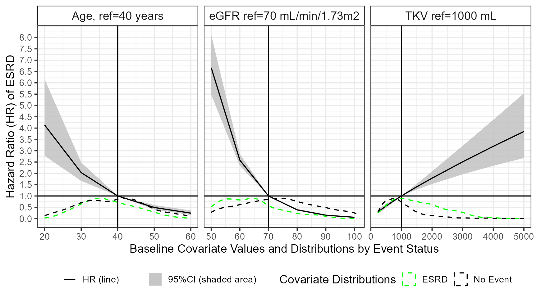
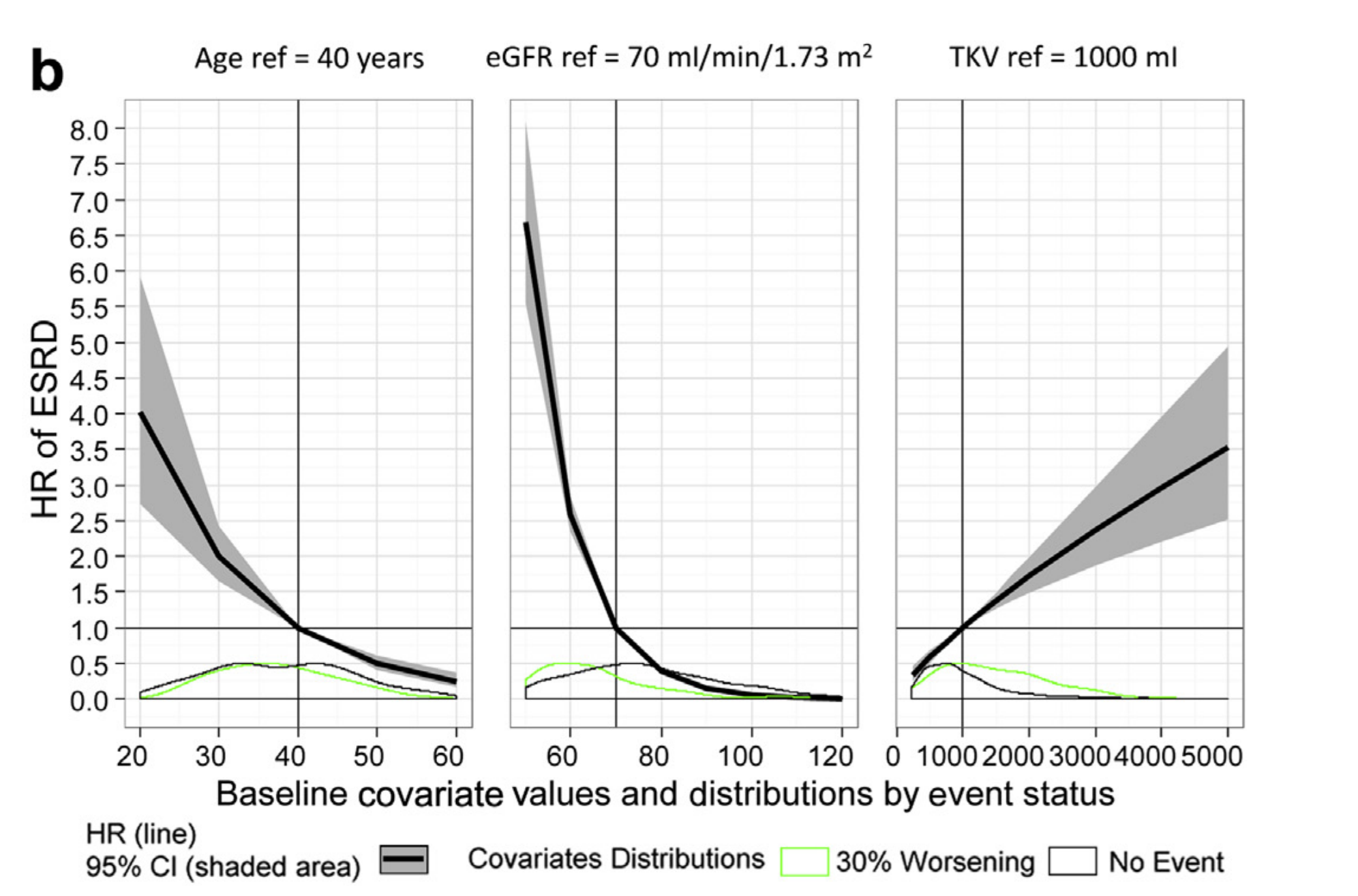
ggplot(matrixhr,aes(x=value,y=HR,ymin=LOW,ymax=HIGH,group=cov) )+
geom_ribbon(aes(fill="95%CI (shaded area)"),alpha=0.8,
color="transparent",
show.legend = c(fill = TRUE, linetype = FALSE))+
geom_vline(aes(xintercept=ref) )+
geom_line(aes(linetype="HR (line)"))+
geom_hline(yintercept = 1 ) +
geom_density(data=covdistribution[covdistribution$status=="1",] ,
aes(y = 0.9*(..scaled..), color="ESRD",
x=value) ,alpha=0.2,inherit.aes = FALSE,linetype="dashed") +
geom_density(data=covdistribution[covdistribution$status=="0",] ,
aes(y = 0.9*(..scaled..),color="No Event",
x=value) ,alpha=0.2,inherit.aes = FALSE,linetype="dashed")+
facet_grid(~cov,scales="free_x") +
scale_y_continuous(breaks=seq(0,8,0.5))+
theme_bw(base_size = 14)+
theme(legend.position="bottom",
strip.background = element_rect(fill = 'white', colour = 'black'),
strip.text.x = element_text(size = 14)) +
xlab("Baseline Covariate Values and Distributions by Event Status")+
ylab("Hazard Ratio (HR) of ESRD")+
labs(colour="Covariate Distributions",
linetype="",fill="")+
scale_fill_manual(values = c("gray"))+
scale_color_manual(values = c("ESRD" = "green","No Event" = "black"))+
guides(linetype = guide_legend(order=1),
fill = guide_legend(order=2,override.aes = list(linetype=NA)),
color = guide_legend(order=3)
)
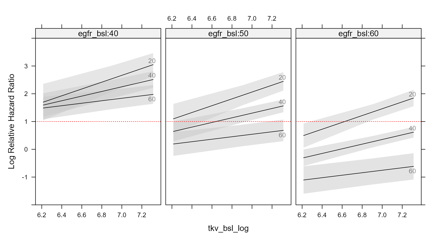
 The code below constructs a grid of values, predict the Hazard Ratios taking into account interactions and use the